
Lesson 1: Introduction to Quantitative Trading
From Market Ideas to Rule-Based, Testable Trading Systems
Quantitative trading is a structured way of making trading decisions using explicit rules, data and measurable evidence.
Instead of relying only on judgement in the moment, a quantitative approach asks whether a market idea can be defined clearly enough to test, repeat and, in some cases, automate.
This does not mean that every quantitative strategy is complex or driven by artificial intelligence. A simple rule based on price, volatility or a moving average can be quantitative if the conditions are objective, consistently applied and evaluated using data.
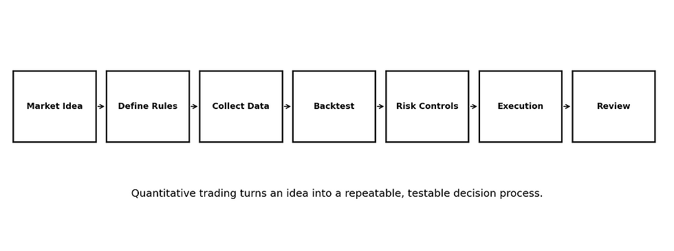
Quantitative trading is less about predicting every market move and more about building a repeatable decision process.
1. What Makes Trading “Quantitative”?
A trading approach becomes quantitative when its decisions can be expressed in measurable terms.
Rather than saying “the market looks strong”, a rule might define strength using a price breakout, a moving-average relationship, a volatility threshold or another observable condition.
The important change is from interpretation to specification. Once a rule is specified, historical data can be used to ask how it would have behaved in different market environments.
2. Quantitative vs Discretionary Trading
Discretionary and quantitative trading are not necessarily opposites.
A discretionary trader may use data and indicators, while a quantitative researcher may still make judgement calls when designing a model. The main difference is where the decision is made.
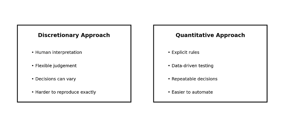
In discretionary trading, the final decision is often made by the trader at the time of execution.
In quantitative trading, more of that decision is transferred into rules before the trade occurs. This makes the process easier to reproduce and test, but it also means that weak assumptions can be repeated systematically.
3. The Building Blocks of a Quant Strategy
A strategy is more than an entry signal.
A complete rule set needs to explain what is traded, when a position can be opened, how large the position should be, when the trade should be ignored and how the position will eventually be closed.

Component | Question | Example |
Universe | What markets are eligible? | A selected group of liquid instruments |
Signal | What creates an opportunity? | Price closes above a defined breakout level |
Filter | When should the signal be ignored? | Volatility is outside the strategy’s allowed range |
Position sizing | How much exposure is taken? | Size is linked to a predefined risk budget |
Exit | What ends the trade? | Stop, target, time rule or opposite signal |
4. From a Trading Idea to a Rule
Suppose the original idea is: “I want to participate when a market begins trending upward.”
That statement is too vague to test. A quantitative version needs observable conditions.
For example, a researcher might define an upward regime as a faster moving average being above a slower moving average.
The rule could then specify exactly when the relationship is checked, what price is used and what additional conditions are required before a position is considered.
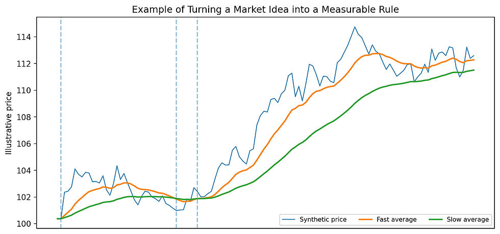
The goal is not to claim that this example is a profitable strategy. It demonstrates how an ambiguous idea can be converted into a testable rule.
5. Data: The Raw Material of Quant Research
Once the rules are clear, the strategy needs data.
Depending on the strategy, this may include:
Open, high, low and close prices
Volume
Spreads
Timestamps
Economic data
Other relevant variables
Data quality matters because a backtest can only be as reliable as the information it receives.
Missing observations, incorrect timestamps, unrealistic prices or inconsistent instrument histories can create misleading results.
Different Frequencies, Different Questions
A daily strategy and a one-minute strategy face very different research problems.
Higher-frequency systems are generally more sensitive to execution assumptions, spreads, latency and data quality. The appropriate dataset should therefore match the intended trading horizon.
6. Backtesting: Replaying the Rules on Historical Data
Backtesting applies the strategy rules to historical data to simulate how the logic would have behaved in the past.
It can reveal:
How frequently signals occurred
How returns were distributed
How large drawdowns became
Whether performance depended heavily on a small number of trades
A backtest is not proof that the strategy will work in the future. It is a research tool for challenging an idea before risking real capital.

In-Sample and Out-of-Sample Thinking
One common research approach is to develop or calibrate the strategy on one portion of historical data and then evaluate it on data that was not used to shape the rules.
The purpose is to reduce the risk of mistaking a good historical fit for a robust trading relationship.
7. Measuring a Strategy
Total return alone does not describe the quality of a strategy.
Two systems can produce similar returns while exposing the trader to very different levels of drawdown, volatility and consistency.

Return
The overall gain or loss generated during the test period.
Maximum Drawdown
The largest peak-to-trough decline, which helps describe the downside experience.
Win Rate
The percentage of trades that are profitable. A high win rate does not automatically mean a strategy is strong.
Profit Factor
A comparison of gross profits with gross losses.
Expectancy
The average amount a strategy is expected to gain or lose per trade based on its historical distribution.
Sharpe Ratio
A commonly used risk-adjusted measure comparing excess return with return variability.
8. Risk Management Is Part of the Model
A quantitative strategy can have a useful signal and still fail if exposure is poorly controlled.
Position sizing, stop logic, portfolio concentration and loss limits should therefore be treated as part of the system rather than added as an afterthought.

For example, the same entry signal can create very different account outcomes when traded with different position sizes.
Quant research therefore needs to evaluate both the signal and the way capital is allocated to that signal.
9. Execution: From Research to the Real Market
A backtest assumes a model of how trades are executed.
Live markets add practical effects such as:
Spreads
Commissions
Slippage
Market gaps
Order restrictions
Changing liquidity
These can create a meaningful difference between a theoretical result and real execution.
Automation through platforms such as MT5 can help apply predefined rules consistently, but automation does not remove these market frictions. The trading program still needs suitable execution logic and risk controls.
10. Common Research Mistakes
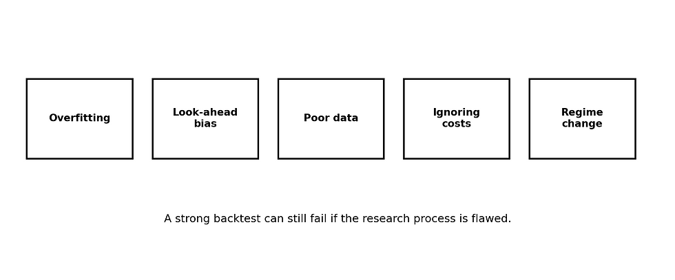
Overfitting
A strategy can become too closely adapted to historical noise, especially when many parameters are repeatedly optimised.
Look-Ahead Bias
A test becomes invalid if it accidentally uses information that would not have been available at the time of the simulated decision.
Poor Data
Missing, incorrect or inconsistent data can produce results that do not reflect the intended market history.
Ignoring Trading Costs
A strategy that trades frequently can look attractive before spreads, commissions and slippage are included.
Regime Change
A relationship that worked in one market environment may weaken when volatility, liquidity or participant behaviour changes.
11. Does Quant Trading Mean Fully Automated Trading?
No. Quantitative trading describes the use of explicit, data-driven rules.
Those rules can be executed manually, semi-automatically or automatically. Automation is an implementation choice.
A researcher may use code only for analysis and backtesting while still placing trades manually.
At the other end of the spectrum, a complete algorithmic system can monitor data, generate signals, size positions and send orders without manual intervention.
12. A Beginner’s Quantitative Trading Workflow
Start with one clear market hypothesis.
Translate the hypothesis into objective rules.
Choose data that matches the intended market and timeframe.
Backtest the rules using realistic assumptions.
Evaluate both return and risk metrics.
Check whether the result survives different periods or parameter choices.
Include transaction costs and execution assumptions.
Define position sizing and account-level risk controls.
Test in a simulated or controlled environment before considering live deployment.
Continue reviewing the strategy as market conditions change.
Key Takeaways
Quantitative trading converts market ideas into measurable and repeatable rules.
A strategy needs more than an entry signal: universe, filters, sizing and exits also matter.
Historical testing is a research tool, not a guarantee of future performance.
Data quality and realistic execution assumptions are essential.
Performance should be evaluated using several return and risk measures.
Risk management is part of the strategy design.
Overfitting, look-ahead bias and trading costs can make a backtest misleading.
Quantitative strategies can be manual, semi-automated or fully automated.
Educational Notice: This material is provided for educational purposes only. It explains general concepts in quantitative and algorithmic trading and does not constitute investment advice, a personal recommendation, or an offer or solicitation to buy or sell any financial instrument. Historical, simulated and backtested results do not guarantee future performance. Trading leveraged products involves significant risk.


Comments